Optim.jl v0.9.0

I am very happy to say that we can finally announce that Optim.jl v0.9.0 is out. This version has quite a few user facing changes. Please read about the changes below if you use Optim.jl in a package, a script, or anything else, as you will quite likely have to make some changes to your code.

As always, I have to thank my two partners in crime: Asbjørn Nilsen Riseth (@anriseth) and Christoph Ortner (@cortner) for their help in making the changes, transitions, and tests that are included in v0.9.0.

The last update (form v0.6.0 to v0.7.0 had) some changes that were a long time coming, and so does v0.9.0. Hopefully, these fixes to old design problems will greatly improve the user experience and performance of Optim.jl, and pave the way for more exiting features in the future.

We’ve tried to make the transition as smooth as possible, although we do have breaking changes in this update. Please consult the documentation if you face problems, join us on gitter or ask the community at discourse!

Okay, now to the changes.

Why not v0.8.0?
First of all, why v0.9.0? Last version was v0.7.8! The is because we are dropping support for Julia v0.4 and v0.5 simultaneously, so we are reserving v0.8.0 for backporting serious fixes to Julia v0.5. However, v0.6 should be just around the corner. With Julia v0.7 and v1.0.0 not too far out in the horizon either, I’ve decided it’s more important to move forward than to keep v0.4 and v0.5 up to speed. The dev time is constrained, so currently it’s one or the other. Of course, for users of Julia v0.5. they can simply continue to use Optim.jl v0.7.8. Post Julia’s proper release, backwards compatibility and continuity will be more important, even if it comes at the expense of development speed.

Another note about the version number: The next version of Optim.jl will be v1.0.0, and we will follow SEMVER 2.0 fully.

Change order of evaluation point and storage arguments
This one is very breaking, although we have set up op a system such that all gradients and Hessians will be checked before proceeding. This check will be removed shortly in a v1.0.0 version bump, so please correct your code now. Basically, we closed a very old issue (#156) concerning the input argument order in gradients and Hessians. In Julia, an in-place function typically has an exclamation mark at the end of its name, and the cache as the first argument. In Optim.jl it has been the other way around for the argument order. We’ve changed that, and this means that you now have to provide “g” or “H” as the first argument, and “x” as the second. The old version

function g!(x, g)
    ... do something ...
end

is now

function g!(g, x)
    ... do something ...
end

NLSolversBase.jl
Since v0.7.0, we’ve moved some of the basic infrastructure of Optim.jl to NLSolversBase.jl. This is currently the Non-, Once-, and TwiceDifferentiable types and constructors. This is done to, as a first step, share code between Optim.jl and LineSearches.jl, and but also NLsolve.jl in the future. At the same time, we’ve made the code a little smarter, such that superfluous calls to the objective function, gradient, and Hessian are now avoided. As an example, compare the objective and gradient calls in the example in our readme. Here, we optimize the Rosenbrock “banana” function using BFGS. Since last version of Optim we had to change the output, as it has gone from 157 calls to 53. Much of this comes from this refactoring, but some of it also comes form a better choices for initial line search steps for BFGS and Newton introduced in #328.

As mentioned, we’ve made the *Differentiable-types a bit smarter, including moving the gradient and Hessian caches into the respective types. This also means, that a OnceDifferentiable type instance needs to know what the return type of the gradient is. This is done by providing an x seed in the constructor

rosenbrock = Optim.UnconstrainedProblems.examples["Rosenbrock"]
f = rosenbrock.f
g! = rosenbrock.g!
x_seed = rosenbrock.initial_x
od = OnceDifferentiable(f, g!, x_seed)

If the seed also happens to be the initial x, then you do not have to provide an x when calling optimize

julia> optimize(od, BFGS(), Optim.Options(g_tol=0.1))
Results of Optimization Algorithm
 * Algorithm: BFGS
 * Starting Point: [1.0005999613152214,1.001138415164852]
 * Minimizer: [1.0005999613152214,1.001138415164852]
 * Minimum: 7.427113e-07
 * Iterations: 13
 * Convergence: true
   * |x - x'| < 1.0e-32: false 
     |x - x'| = 1.08e-02 
   * |f(x) - f(x')| / |f(x)| < 1.0e-32: false
     |f(x) - f(x')| / |f(x)| = NaN 
   * |g(x)| < 1.0e-01: true 
     |g(x)| = 2.60e-02 
   * stopped by an increasing objective: false
   * Reached Maximum Number of Iterations: false
 * Objective Calls: 45
 * Gradient Calls: 45

If you’ve used Optim.jl before, you’ll notice that the output carries a bit more information about the convergence criteria.

LineSearches.jl turned Julian
Line searches used to be chosen using symbols in the method constructor for line search based methods such as GradientDescent, BFGS, and Newton by use of the linesearch keyword. The new version of LineSearches.jl uses types and dispatch exactly like Optim.jl does for solvers. This means that you now have to pass a type instance instead of a keyword, and this also means that we can open up for easy tweaking of line search parameters through fields in the line search types.

Let us illustrate by the following example how the new syntax works. First, we construct a BFGS instance without specifying the linesearch. This defaults to HagerZhang.

julia> rosenbrock(x) =  (1.0 - x[1])^2 + 100.0 * (x[2] - x[1]^2)^2
rosenbrock (generic function with 1 method)
 
julia> result = optimize(rosenbrock, zeros(2), BFGS())
Results of Optimization Algorithm
 * Algorithm: BFGS
 * Starting Point: [0.0,0.0]
 * Minimizer: [0.9999999926033423,0.9999999852005353]
 * Minimum: 5.471433e-17
 * Iterations: 16
 * Convergence: true
   * |x - x'| < 1.0e-32: false
     |x - x'| = 3.47e-07
   * |f(x) - f(x')| / |f(x)| < 1.0e-32: false
     |f(x) - f(x')| / |f(x)| = NaN
   * |g(x)| < 1.0e-08: true
     |g(x)| = 2.33e-09
   * stopped by an increasing objective: false
   * Reached Maximum Number of Iterations: false
 * Objective Calls: 53
 * Gradient Calls: 53

or we could choose a backtracking line search instead

 
julia> optimize(rosenbrock, zeros(2), BFGS(linesearch = LineSearches.BackTracking()))
Results of Optimization Algorithm
 * Algorithm: BFGS
 * Starting Point: [0.0,0.0]
 * Minimizer: [0.9999999926655744,0.9999999853309254]
 * Minimum: 5.379380e-17
 * Iterations: 23
 * Convergence: true
   * |x - x'| < 1.0e-32: false
     |x - x'| = 1.13e-09
   * |f(x) - f(x')| / |f(x)| < 1.0e-32: false
     |f(x) - f(x')| / |f(x)| = NaN
   * |g(x)| < 1.0e-08: true
     |g(x)| = 8.79e-11
   * stopped by an increasing objective: false
   * Reached Maximum Number of Iterations: false
 * Objective Calls: 31
 * Gradient Calls: 24

this defaults to cubic backtracking, but quadratic can be chosen using the order keyword

julia> optimize(rosenbrock, zeros(2), BFGS(linesearch = LineSearches.BackTracking(order = 2)))
Results of Optimization Algorithm
 * Algorithm: BFGS
 * Starting Point: [0.0,0.0]
 * Minimizer: [0.9999999926644578,0.9999999853284671]
 * Minimum: 5.381020e-17
 * Iterations: 23
 * Convergence: true
   * |x - x'| < 1.0e-32: false
     |x - x'| = 4.73e-09
   * |f(x) - f(x')| / |f(x)| < 1.0e-32: false
     |f(x) - f(x')| / |f(x)| = NaN
   * |g(x)| < 1.0e-08: true
     |g(x)| = 1.76e-10
   * stopped by an increasing objective: false
   * Reached Maximum Number of Iterations: false
 * Objective Calls: 29
 * Gradient Calls: 24

LineSearches.jl should have better documentation coming soon, but the code is quite self-explanatory for those who want to twiddle around with these parameters.

The method state is now an argument to optimize
While not always that useful to know for users, we use method states internally to hold all the pre-allocated cache variables that are needed. In the new version of Optim.jl, this can be explicitly provided by the user such that you can retrieve various diagnostics after the optimization routine is done. One such example is the inverse Hessian estimate that BFGS spits out.

method = BFGS()
options = Optim.Options()
initial_x = rand(2)
d = OnceDifferentiable(f, g!, initial_x)
my_state = Optim.initial_state(method, options, d, initial_x)
optimize{d, method, options, my_state)

The future
We have more changes coming in the near future. There’s PR #356 for a Trust Region solver for cases where you can explicitly calculate Hessian-vector products without forming the Hessian (from @jeff-regier from the Celeste.jl project), the interior point replacement for our current barrier function approach to box constrained optimization in PR #303, and more.
Solving a simple discrete choice model using Gaussian quadrature

In the style of some of the earlier posts, I present a simple economic problem, that uses some sort of numerical method as part of the solution method. Of course, we use Julia to do so. However, this time we’re actually relying a bit on R, but don’t tell anyone.

Rust models

In the empirical discrete choice literature in economics, a relatively simple and popular framework is the one that matured in Rust (1987, 1988), and was later named Rust models in Aguirregabiria and Mira (2010). Basically, we consider an agent who has to choose a (in the infinite horizon) stationary policy (sequence of actions), to solve the following problem

\(\max_{a}E\left\{\sum_{t=0}^{T} \beta^t U(a_t, s_t)|s_0\right\}\)

where \(a=(a_0, a_1, \ldots, a_T)\), and \(s_t\) denotes the states. For simplicity, we consider binary decision problems such that \(a_t\in\{1,2\}\). Assume that there an additive shock, \(\varepsilon_t\), to utility such that

\(U(a_t,s_t)=U(a_t, x_t, \varepsilon_t) = u(a_t, x_t)+\varepsilon_t\)

where \(s_t=(x_t,\varepsilon_t)\) and \(x_t\) is usually called the observed states.

The additive and time separable nature of the problem allows us to consider a set of simpler problems instead. We reformulate the problem according to the principle of optimality, and write the problem in its dynamic programming formulation

\( V_t(x_t, \varepsilon_t) = max_{a_t}\left[u(a_t, x_t)+\epsilon_t + \beta E_{s_{t+1}|s_t}(V_{t+1}(x_{t+1}, \varepsilon_{t+1}))\right], \forall t\in\{0,1,\ldots,T\} \)

The object \(V_t\) is called the value function, as it summarizes the optimal value we can obtain. If we assume conditional independence between the observed states and the shocks along with the assumptions explained in the articles above, we can instead consider this simpler problem

\( W_t(x_t) = E_{\varepsilon_{t+1}|\varepsilon_t}\left\{max_{a_t}(u(a_t, x_t)+\varepsilon_t + \beta E_{x_{t+1}|x_t}((W_{t+1}(x_{t+1}))\right\}, \forall t\in\{0,1,\ldots,T\} \)

where \(W(x_t)\equiv E_{\varepsilon_{t+1}|\varepsilon}\left\{V_{t+1}(x_{t+1},\varepsilon_{t+1})\right\}\). This object is often called the ex-ante or integrated value function. Now, if we assume that the shocks are mean 0 extreme value type I, we get the following

\( W_t(x_t) = \log\left\{\sum_{a\in\mathcal{A}} \exp\left[u(a_t,x_t)+\beta E_{x_{t+1}|x_t}\left(W_{t+1}(x_{t+1})\right)\right]\right\}, \forall t\in\{0,1,\ldots,T\} \)

At this point we’re very close to something we can calculate. Either we just recursively apply the above to find the finite horizon solution, or if we’re in the infinite horizon case, then then we can come up with a guess for \(W\), and apply value function iterations (successive application of the right-hand side in the equation above), to find a solution. We just need to be able to handle the evaluation of the expected value inside the \(\exp\)‘s.

Solving for a continuous function

In the application below, we’re going to have a continuous state. Rust originally solved the problem of handling a continuous function on a computer by discretizing the continuous state in 90 or 175 bins, but we’re going to approach it a bit differently. We’re going to create a type that allows us to construct piecewise linear functions. This means that we’re going to have some nodes where we calculate the function value, and in between these, we simply use linear interpolation. Outside of the first and last nodes we simply set the value to the value at these nodes. We’re not going to extrapolate below, so this won’t be a problem.

Let us have a look at a type that can hold this information.

type PiecewiseLinear
    nodes
    values
    slopes
end

To construct an instance of this type from a set of nodes and a function, we’re going to use the following constructor

function PiecewiseLinear(nodes, f)
    slopes = Float64[]
    fn = f.(nodes)
    for i = 1:length(nodes)-1
        # node i and node i+1
        ni, nip1 = nodes[i], nodes[i+1]
        # f evaluated at the nodes
        fi, fip1 = fn[i], fn[i+1]
        # store slopes in each interval, so we don't have to recalculate them every time
        push!(slopes, (fip1-fi)/(nip1-ni))
    end
    # Construct the type
    PiecewiseLinear(nodes, fn, slopes)
end

Using an instance of \(PiecewiseLinear\) we can now evaluate the function at all input values between the first and last nodes. However, we’re going to have some fun with types in Julia. In Julia, we call a function using parentheses \(f(x)\), but we generally cannot call a type instance.

julia> pwl = PiecewiseLinear(1:10, sqrt)
PiecewiseLinear(1:10,[1.0,1.41421,1.73205,2.0,2.23607,2.44949,2.64575,2.82843,3.0,3.16228],[0.414214,0.317837,0.267949,0.236068,0.213422,0.196262,0.182676,0.171573,0.162278])
 
julia> pwl(3.5)
ERROR: MethodError: objects of type PiecewiseLinear are not callable

… but wouldn’t it be great if we could simply evaluate the interpolated function value at 3.5 that easily? We can, and it’s cool, fun, and extremely handy. The name of the concept is: call overloading. We simply need to define the behavior of “calling” (using parentheses with some input) an instance of a type.

function (p::PiecewiseLinear)(x)
    index_low = searchsortedlast(p.nodes, x)
    n = length(p.nodes)
    if 0 < index_low < n
        return p.values[index_low+1]+(x-p.nodes[index_low+1])*p.slopes[index_low]
    elseif index_low == n
        return p.values[end]
    elseif index_low == 0
        return p.values[1]
    end
end

Basically, we find out which interval we’re in, and then we interpolate appropriately in said interval. Let me say something upfront, or… almost upfront. This post is not about optimal performance. Julia is often sold as “the fast language”, but to me Julia is much more about productivity. Sure, it’s great to be able to optimize your code, but it’s also great to simply be able to do *what you want to do* – without too much hassle. Now, we can do what we couldn’t before.

julia> pwl(3.5)
1.8660254037844386

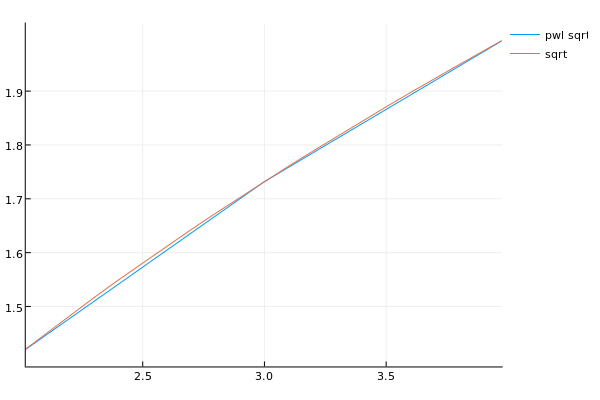
We can even plot it together with the actual sqrt function on the interval (2,4).

julia> using Plots
 
julia> plot(x->pwl(x), 2, 4, label="Piecewise Linear sqrt")
 
julia> plot!(sqrt, 2, 4, label="sqrt")
 
julia> savefig("sqrtfig")

and we get

which seems to show a pretty good approximation to the square root function considering the very few nodes.

Numerical integrals using Gaussian quadrature

So we can now create continuous function approximations based on finite evaluation points (nodes). This is great, because this allow us to work with \(W\) in our code. The only remaining problem is: we need to evaluate the expected value of \(W\). This can be expressed as

\( E_x(f) = \int_a^b f(x)w(x)dx\)

where \(w(x)\) is going to be a probability density function and \(a\) and \(b\) can be finite or infinite and represent upper and lower bounds on the values the random variable (state) can take on. In the world of Gaussian quadrature, \(w\)‘s are called weight functions. Gaussian quadrature is basically a method for finding good evaluation points (nodes) and associated weights such that the following approximation is good

\(\int_a^b f(x)w(x)dx\approx \sum_{i=1}^N f(x_i)w_i\)

where \(N\) is the number of nodes. We’re not going to provide a long description of the methods involved, but we will note that the package DistQuads.jl allows us to easily obtain nodes and weights for a handful of useful distributions. To install this package write

Pkg.clone("https://github.com/pkofod/DistQuads.jl.git")

as it is not currently tagged in METADATA.jl. This is currently calling out to R’s statmod package. The syntax is quite simple. Define a distribution instance, create nodes and weights, and calculate the expected value of the function in three simple steps:

julia> using Distributions, DistQuads
 
julia> bd = Beta(1.5, 50.0)
Distributions.Beta{Float64}(α=1.5, β=50.0)
 
julia> dq = DistQuad(bd, N = 64)
DistQuads.DistQuad([0.000334965,0.00133945,0.00301221,0.0053512,0.00835354,0.0120155,0.0163327,0.0212996,0.0269103,0.03315780.738325,0.756581,0.774681,0.792633,0.810457,0.828194,0.845925,0.863807,0.882192,0.902105],[0.00484732,0.0184431,0.0381754,0.0603806,0.0811675,0.097227,0.106423,0.108048,0.102724,0.0920435  …  1.87035e-28,5.42631e-30,1.23487e-31,2.11992e-33,2.60541e-35,2.13019e-37,1.03855e-39,2.52575e-42,2.18831e-45,2.90458e-49],Distributions.Beta{Float64}(α=1.5, β=50.0))
 
julia> E(sqrt, dq)
0.15761865929803381

We can then try Monte Carlo integration with many nodes to see how close they are

julia> mean(sqrt.(rand(bd, 100000000)))
0.1576136243615477

and they appear to be in the same ballpark.

To replace, or not to replace

The model we’re considering here is a simple one. It’s a binary choice model very close to the model in Rust (1987). An agent is in charge of maintaining a bus fleet and has a binary choice each month then the buses come in for maintenance: replace the engine (effectively renewing the bus) or maintain it. Replacement costs a fixed price RC, and regular maintenance has a cost that is a linear function of the odometer reading since last replacement (or purchase if replacement has never occurred). We can use the expressions above to solve this model, but first we need to specify how the odometer reading changes from month to month conditional on the choices made. We assume that the odometer reading (mileage) changes according to the following

\(x_{t+1}=\tilde{a}x_{t}+(1-\tilde{a}x_t)\Delta x, \quad\text{where }\Delta x \sim Beta(1.4, 50.0)\)

where \(\tilde{a}=2-a\), and as we remember \(a\in\{1,2\}\). As we see, a replacement returns the state to 0 plus whatever mileage might accumulate that month, and regular maintenance means that the bus will end up with end of period mileage between \(x_{t+1}\) and 1. To give an idea about the state process, we see the pdf for the distribution of \(\Delta x\) below.

Solving the model

We are now ready to solve the model. Let us say that the planning horizon is 96 months and the monthly discount factor is 0.9. After the 96 months, the bus is scrapped at a value of 2 units of currency, such that

\(W_T(x)=2.0\)

and from here on, we use the recursion from above. First, set up the state space.

using Distributions, DistQuads, Plots
# State space
bd = Beta(1.5, 50.0)
dq = DistQuad(bd, N = 64)
 
Sˡ = 0
Sʰ = 1
 
n_nodes = 100 # arbitrary, but could be varied
nodes = linspace(Sˡ, Sʰ, n_nodes) # doesn't have to be uniformly distributed
 
RC = 11.5 # Replacement cost
c = 9.0 # parameter in linear maintenance cost c*x
β = 0.9 # discount factor

Then, define utility function and expectation operator

u1 = PiecewiseLinear(nodes, x->-c*x) # "continuous" cost of maintenance
u2 = PiecewiseLinear(nodes, x->-RC) # "continuous" cost of replacement (really just a number, but...)
 
# Expected value of f at x today given a where x′ is a possible state next period
Ex(f, x, a, dq) = E(x′->f((2-a)*x.+(Sʰ-(2-a)*x).*x′), dq)

Then, we simply

#### SOLVE
V = Array{PiecewiseLinear,1}(70)
V[70] = PiecewiseLinear(nodes, x->2)
for i = 69:-1:1
    EV1 = PiecewiseLinear(nodes, x->Ex(V[i+1], x, 1, dq))
    EV2 = PiecewiseLinear(nodes, x->Ex(V[i+1], x, 2, dq))
    V[i] = PiecewiseLinear(nodes, x->log(exp(u1(x)*EV1(x))+exp(u2(x)*EV2(x))))
end

To get our solution. We can then plot either integrated value functions or policies (choice probabilities). We calculate the policies using the following function

function CCP(x, i)
    EV1 = PiecewiseLinear(nodes, x->Ex(V[i], x, 1, dq))
    EV2 = PiecewiseLinear(nodes, x->Ex(V[i], x, 2, dq))
    1/(1+exp(u2(x)*EV2(x)-u1(x)*EV1(x)))
end


We see that there are not 69/70 distinct curves in the plots. This is because we eventually approach the “infinite horizon”/stationary policy and solution.

Simulation

Given the CCPs from above, it is very straight forward to simulate an agent say from period 1 to period 69.

#### SIMULATE
x0 = 0.0
x = [x0]
a0 = 0
a = [a0]
T = 69
for i = 2:T
   _a = rand()<CCP(x[end], i) ? 1 : 2
   push!(a, _a)
   push!(x, (2-_a)*x[end]+(Sʰ-(2-_a)*x[end])*rand(bd))
end
plot(1:T, x, label="mileage")
Is = []
for i in eachindex(a)
    if a[i] == 2
        push!(Is, i)
    end
end
vline!(Is, label="replacement")


Conclusion
This blog post had a look at simple quadrature, creating custom types with call overloading in Julia, and how this can be used to a solve a very simple discrete choice model in Julia. Interesting extensions are of course to allow for more states, more choices, other shock distributions than extreme value type I and so on. Let me know if you try to extend the model in any of those directions, and I would love to have a look!

References

  • Aguirregabiria, Victor, and Pedro Mira. “Dynamic discrete choice structural models: A survey.” Journal of Econometrics 156.1 (2010): 38-67.
  • Rust, John. “Optimal replacement of GMC bus engines: An empirical model of Harold Zurcher.” Econometrica: Journal of the Econometric Society (1987): 999-1033.
  • John, Rust. “Maximum likelihood estimation of discrete control processes.” SIAM Journal on Control and Optimization 26.5 (1988): 1006-1024.
  • Timing in Julia

    Timing code is important when you want to benchmark or profile your code. Is it the solution of a linear system or the Monte Carlo integration scheme that takes up most of the time? Is version A or version B of a function faster? Questions like that show up all the time. Let us have a look at a few of the possible ways of timing things in Julia.

    The basics

    The most basic timing functionalities in Julia are the ones included in the Base language. The standard way of timing things in Julia, is by use of the @time macro.

    julia> function test(n)
               A = rand(n, n)
               b = rand(n)
               @time A\b
           end
    test (generic function with 1 method)

    Do note, that the code we want to time is put in a function . This is because everything we do at the top level in the REPL is in global scope. It’s a mistake a lot of people do all the time, but currently it is a very bad idea performance wise. Anyway, let’s see what happens for n = 1, 10, 100, and 1000.

    julia> test(1);
      0.000002 seconds (7 allocations: 320 bytes)
     
    julia> test(10);
      0.000057 seconds (9 allocations: 1.313 KB)
     
    julia> test(100);
      0.001425 seconds (10 allocations: 80.078 KB)
     
    julia> test(1000);
      0.033573 seconds (10 allocations: 7.645 MB, 27.81% gc time)
     
    julia> test(1000);
      0.045214 seconds (10 allocations: 7.645 MB, 47.66% gc time)

    The first run is to compile both test, and then we have a look at what happens when the dimension of our problem increases. Elapsed time seems to increase, and we also see that the number of allocations, and the amount of memory that was allocated increases. For the runs with dimension 1000 we see something else in the output. 30-50% of the time was spent in “gc”. What is this? Julia is a garbage collected language. This means that Julia keeps track of current allocations, and frees the memory if it isn’t needed anymore. It doesn’t do this all the time, though. Running the 1000-dimensional problem once more gives us

    julia> test(1000)
      0.029277 seconds (10 allocations: 7.645 MB)

    We see it runs slightly faster, and there is no GC time this time around. Of course, these things will look slightly different if you try to replicate them.

    So now we can time. But what if we want to store this number? We could be tempted to try

    t = @time 3+3

    but we will realize, that what is returned is the return value of the expression, not the elapsed time. To save the time, we can either use @timed or @elapsed. Let us try to change the @time to @timed and look at the output when we have our new test2 function return the return value.

    julia> function test2(n)
               A = rand(n, n)
               b = rand(n)
               @timed A\b
           end
    test2 (generic function with 1 method)
     
    julia> test2(3)
    ([0.700921,-0.120765,0.683945],2.7889e-5,512,0.0,Base.GC_Diff(512,0,0,9,0,0,0,0,0))

    We see that it returns a tuple with: the return value of A\b followed by the elapsed time, then the bytes allocated, time spent in garbage collection, and lastly some further memory counters. This is great as we can now work with the information @time printed, but we still have access to the results of our calculations. Of course, it is a bit involved to do it this way. If we simply wanted to see the elapsed time to act on that – then we would just use @time as we did above.

    Before we move on to some simpler macros, let us consider the last “time*-family” macro: @timev. As we saw above, @timed contained more information about memory allocation than @time printed. If we want the “verbose” version, we use @timev (v for verbose):

    julia> function test3(n)
               A = rand(n, n)
               b = rand(n)
               @timev A\b
           end
    test3 (generic function with 1 method)

    Running test3 on a kinda large problem, we see that is does indeed print the contents of Base.GC_Diff

    julia> test3(5000);
      1.923164 seconds (12 allocations: 190.812 MB, 4.67% gc time)
    elapsed time (ns): 1923164359
    gc time (ns):      89733440
    bytes allocated:   200080368
    pool allocs:       9
    malloc() calls:    3
    GC pauses:         1
    full collections:  1

    If any of the entries are zero, the corresponding lines are omitted.

    julia> test3(50);
      0.001803 seconds (10 allocations: 20.828 KB)
    elapsed time (ns): 1802811
    bytes allocated:   21328
    pool allocs:       9
    malloc() calls:    1

    Of the three macros, you’ll probably not use @timev a lot.

    Simpler versions

    If we only want the elapsed time or only want the allocations, then we used either the @elapsed or @allocated macros. However, these do not return the results of our calculations, so in many cases it may be easier to just used @timed, so we can grab the results, the elapsed time, and the allocation information. “MATLAB”-style tic();toc()‘s are also available. toc() prints the time, while toq() is used if we want only the returned time without the printing. It is also possible to use time_ns() to do what time.time() would do in Python, although for practically all purposes, the above macros are recommended.

    More advanced functionality

    Moving on to more advanced features, we venture into the package ecosystem.

    Nested timings

    The first package I will present is the nifty TimerOutputs.jl by Kristoffer Carlsson. This packages essentially allows you to nest @time calls. The simplest way to show how it works, is to use the example posted at the announcement (so credit to Kristoffer for the example).

    using TimerOutputs
     
    # Create the timer object
    to = TimerOutput()
     
    # Time something with an assigned label
    @timeit to "sleep" sleep(0.3)
     
    # Data is accumulated for multiple calls
    for i in 1:100
        @timeit to "loop" 1+1
    end
     
    # Nested sections are possible
    @timeit to "nest 1" begin
        @timeit to "nest 2" begin
            @timeit to "nest 3.1" rand(10^3)
            @timeit to "nest 3.2" rand(10^4)
            @timeit to "nest 3.3" rand(10^5)
        end
        rand(10^6)
    end

    Basically we’re timing the sleep call in one time counter, all the additions in the loop in another counter, and then we do some nested generation of random numbers. Displaying the to instance gives us something like the following

     ───────────────────────────────────────────────────────────────────────
                                    Time                   Allocations      
                            ──────────────────────   ───────────────────────
        Tot / % measured:        6.48s / 5.60%           77.4MiB / 12.0%    
     
     Section        ncalls     time   %tot     avg     alloc   %tot      avg
     ───────────────────────────────────────────────────────────────────────
     sleep               1    338ms  93.2%   338ms    804KiB  8.43%   804KiB
     nest 1              1   24.7ms  6.80%  24.7ms   8.52MiB  91.5%  8.52MiB
       nest 2            1   9.10ms  2.51%  9.10ms    899KiB  9.43%   899KiB
         nest 3.1        1   3.27ms  0.90%  3.27ms   8.67KiB  0.09%  8.67KiB
         nest 3.3        1   3.05ms  0.84%  3.05ms    796KiB  8.34%   796KiB
         nest 3.2        1   2.68ms  0.74%  2.68ms   92.4KiB  0.97%  92.4KiB
     loop              100   6.97μs  0.00%  69.7ns   6.08KiB  0.06%      62B
     ───────────────────────────────────────────────────────────────────────

    which nicely summarizes absolute and relative time and memory allocation of the individual @timeit calls. A real use case could be to see what the effect is of using finite differencing to construct the gradient for the Generalized Rosenbrock (GENROSEN) problem from CUTEst.jl using a conjugate gradient solver in Optim.jl.

    using CUTEst, Optim, TimerOutputs
     
    nlp = CUTEstModel("GENROSE")
     
    const to = TimerOutput()
     
    f(x    ) =  @timeit to "f"  obj(nlp, x)
    g!(g, x) =  @timeit to "g!" grad!(nlp, x, g)
     
    begin
    reset_timer!(to)
    @timeit to "Conjugate Gradient" begin
        res = optimize(f, g!, nlp.meta.x0, ConjugateGradient(), Optim.Options(iterations=5*10^10));
        println(Optim.minimum(res))
    end
    @timeit to "Conjugate Gradient (FiniteDiff)" begin
        res = optimize(f, nlp.meta.x0, ConjugateGradient(), Optim.Options(iterations=5*10^10));
        println(Optim.minimum(res))
    end
    show(to; allocations = false)
    end

    the output is a table as before, this time without the allocations (notice the use of the allocations keyword in the show method)

     ────────────────────────────────────────────────────────────────
                                                       Time          
                                               ──────────────────────
                 Tot / % measured:                  33.3s / 100%     
     
     Section                           ncalls     time   %tot     avg
     ────────────────────────────────────────────────────────────────
     Conjugate Gradient (FiniteDiff)        1    33.2s  99.5%   33.2s
       f                                1.67M    32.6s  97.9%  19.5μs
     Conjugate Gradient                     1    166ms  0.50%   166ms
       g!                               1.72k   90.3ms  0.27%  52.6μs
       f                                2.80k   59.1ms  0.18%  21.1μs
     ────────────────────────────────────────────────────────────────

    And we conclude: finite differencing is very slow when you’re solving a 500 dimensional unconstrained optimization problem, and you really want to use the analytical gradient if possible.

    Benchmarking

    Timing individual pieces of code can be very helpful, but when we’re timing small function calls, this way of measuring performance can be heavily influenced by noise. To remedy that, we use proper benchmarking tools. The package for that, well, it’s called BenchmarkTools.jl and is mainly written by Jarrett Revels. The package is quite advanced in its feature set, but its basic functionality is straight forward to use. Please see the manual for more details than we provide here.

    Up until now, we’ve asked Julia to tell us how much time some code took to run. Unfortunately for us, the computer is doing lots of stuff besides the raw calculations we’re trying to time. From the example earlier, this means that we have a lot of noise in our measure of the time it takes to solve A\b. Let us try to run test(1000) a few times

    julia> test(1000);
      0.029859 seconds (10 allocations: 7.645 MB)
     
    julia> test(1000);
      0.033381 seconds (10 allocations: 7.645 MB, 6.41% gc time)
     
    julia> test(1000);
      0.024345 seconds (10 allocations: 7.645 MB)
     
    julia> test(1000);
      0.039585 seconds (10 allocations: 7.645 MB)
     
    julia> test(1000);
      0.037154 seconds (10 allocations: 7.645 MB, 2.82% gc time)
     
    julia> test(1000);
      0.024574 seconds (10 allocations: 7.645 MB)
     
    julia> test(1000);
      0.022185 seconds (10 allocations: 7.645 MB)

    There’s a lot of variance here! Let’s benchmark instead. The @benchmark macro won’t work inside a function as above. This means that we have to be a bit careful (thanks to Fengyang Wang for clarifying this). Consider the following

    julia> n = 200;
     
    julia> A = rand(n,n);
     
    julia> b = rand(n);
     
    julia> @benchmark A\b
    BenchmarkTools.Trial: 
      memory estimate:  316.23 KiB
      allocs estimate:  10
      --------------
      minimum time:     531.227 μs (0.00% GC)
      median time:      718.527 μs (0.00% GC)
      mean time:        874.044 μs (3.12% GC)
      maximum time:     95.515 ms (0.00% GC)
      --------------
      samples:          5602
      evals/sample:     1

    This is fine, but since A and b are globals (remember, if it ain’t wrapped in a function, it’s a global when you’re working from the REPL), we’re also measuring the time dynamic dispatch takes. Dynamic dispatch happens here, because “Julia” cannot be sure what the types of A and b are when we invoke A\b since they’re globals. Instead, we should use interpolation of the non-constant variables, or mark them as constants using const A = rand(n,n) and const b = rand(20). Let us use interpolation.

    julia> @benchmark $A\$b
    BenchmarkTools.Trial: 
      memory estimate:  316.23 KiB
      allocs estimate:  10
      --------------
      minimum time:     531.746 μs (0.00% GC)
      median time:      717.269 μs (0.00% GC)
      mean time:        786.240 μs (3.22% GC)
      maximum time:     12.463 ms (0.00% GC)
      --------------
      samples:          6230
      evals/sample:     1

    We see that the memory information is identical to the information we got from the other macros, but we now get a much more robust estimate of the time it takes to solve our A\b problem. We also see that dynamic dispatch was negligible here, as the solution takes much longer to compute than for Julia to figure out which method to call. The @benchmark macro will do various things automatically, to try to give as accurate results as possible. It is also possible to provide custom tuning parameters, say if you’re running these benchmarks over an extended period of time and want to track performance regressions, but that is beyond this blog post.

    Dynamic dispatch

    Before we conclude, let’s have a closer look at the significance of dynamic dispatch. When using globals it has to be determined at run time which method to call. If there a few methods, this may not be a problem, but the problem begins to show itself when a function has a lot of methods. For example, on Julia v0.5.0, identity has one method, but + has 291 methods. Can we measure the significance of dynamic dispatch then? Sure. Just benchmark with, and without interpolation (thanks again to Fengyang Wang for cooking up this example). To keep output from being too verbose, we’ll use the @btime macro – again from BenchmarkTools.jl (there is also an @belapsed that returns the minimum time in seconds).

    julia> x = 0
    0
     
    julia> @btime identity(x)
      1.540 ns (0 allocations: 0 bytes)
    0
     
    julia> @btime +x
      15.837 ns (0 allocations: 0 bytes)
    0
     
    julia> @btime identity($x)
      1.540 ns (0 allocations: 0 bytes)
    0
     
    julia> @btime +$x
      1.548 ns (0 allocations: 0 bytes)
    0

    As we can see, calling + on the global x takes around 10 times a long as the single method function identity. To show that declaring the input a const and interpolating the variable gives the same result, consider the example below.

    julia> const y = 0
    0
     
    julia> @btime identity(y)
      1.539 ns (0 allocations: 0 bytes)
    0
     
    julia> @btime +y
      1.540 ns (0 allocations: 0 bytes)
    0
     
    julia> @btime identity($y)
      1.540 ns (0 allocations: 0 bytes)
    0
     
    julia> @btime +$y
      1.540 ns (0 allocations: 0 bytes)
    0

    We see that interpolation is not needed, as long as we remember to use constants.

    Conclusion

    There are quite a few ways of measuring performance in Julia. I’ve presented some of them here, and hopefully you’ll be able to put the tools to good use. The functionality from Base is good for many purposes, but I really like the nested time measuring in TimerOutputs.jl a lot, and for serious benchmarking it is impossible to ignore BenchmarkTools.jl.

    DynProg Class – Week 2

    This post, and other posts with similar tags and headers, are mainly directed at the students who are following the Dynamic Programming course at Dept. of Economics, University of Copenhagen in the Spring 2017. The course is taught using Matlab, but I will provide a few pointers as to how you can use Julia to solve the same problems. So if you are an outsider reading this I welcome you, but you won’t find all the explanations and theory here. If you want that, you’ll have to come visit us at UCPH and enroll in the class!

    This week we continue with a continuous choice model. This means we have to use interpolation and numerical optimization.

    A (slightly less) simple model

    Consider a simple continuous choice consumption-savings model:

    \(V_t(M_t) = \max_{C_t}\sqrt{C_t}+\mathbb{E}[V_{t+1}(M_{t+1})|C_t, M_t]\)
    subject to
    \(M_{t+1} = M_t – C_t+R_t\\
    C_t\leq M_t\\
    C_t\in\mathbb{R}_+\)

    where \(R_t\) is 1 with probability \(\pi\) and 0 with probability \(1-\pi\), \(\beta=0.9\), and \(\bar{M}=5\)

    Last week the maximization step was merely comparing values associated with the different discrete choices. This time we have to do continuous optimization in each time period. Since the problem is now continuous, we cannot solve for all \(M_t\). Instead, we need to solve for \(V_t\) at specific values of \(M_t\), and interpolate in between. Another difference to last time is the fact that the transitions are stochastic, so we need to form (very simple) expectations as part of the Bellman equation evaluations.

    Interpolation

    It is of course always possible to make your own simple interpolation scheme, but we will use the functionality provided by the Interpolations.jl package. To perform interpolation, we need a grid to be used for interpolation \(\bar{x}\), and calculate the associated function values.

    f(x) = (x-3)^2
    x̄ = linspace(1,5,5)
    fx̄ = f.()

    Like last time, we remember that the dot after the function name and before the parentheses represent a “vectorized” call, or a broadcast – that is we call f on each element of the input. We now use the Interpolations.jl package to create an interpolant \(\hat{f}\).

    using Interpolations
    f̂ = interpolate((collect(),), fx̄, Gridded(Linear()))

    We can now index into \(\hat{f}\) as if it was an array

    [-3] #returns 16.0

    We can also plot it

    using Plots
    plot()

    which will output

    Solving the model

    Like last time, we prepare some functions, variables, and empty containers (Arrays)

    # Model again
    u(c) = sqrt(c)
    T = 10; β = 0.9
    π = 0.5 ;M₁ = 5
    # Number of interpolation nodes
    Nᵐ = 50 # number of grid points in M grid
    Nᶜ  = 50 # number of grid points in C grid
     
    M = Array{Vector{Float64}}(T)
    V = Array{Any}(T)
    C = Array{Any}(T)

    The V and C arrays are allocated using the type “Any”. We will later look at how this can hurt performance, but for now we will simply do the convenient thing. Then we solve the last period

    M[T] = linspace(0,M₁+T,Nᵐ)
    C[T] = M[T]
    V[T] = interpolate((M[T],), u.(C[T]), Gridded(Linear()))

    This new thing here is that we are not just saving V[T] as an Array. The last element is the interpolant, such that we can simply index into V[T] as if we had the exact solution at all values of M (although we have to remember that it is an approximation). For all periods prior to T, we have to find the maximum as in the Bellman equation from above. To solve this reduced “two-period” problem (sum of utility today and discounted value tomorrow), we need to form expectations over the two possible state transitions given an M and a C today, and then we need to find the value of C that maximizes current value. We define the following function to handle this

    # Create function that returns the value given a choice, state, and period
    v(c, m, t, V) = u(c)*(π*V[t+1][m-c+1]+(1)*V[t+1][m-c])

    Notice how convenient it is to simply index into V[t] using the values we want to evaluate tomorrow’s value function at. We perform the maximization using grid search on a predefined grid from 0 to the particular M we’re solving form. If we abstract away from the interpolation step, this is exactly what we did last time.

    for t = T-1:-1:1
        M[t] = linspace(0,M₁+t,Nᵐ)
        C[t] = zeros(M[t])
        Vt = fill(-Inf, length(M[t]))
        for (iₘ, m) = enumerate(M[t])
            for c in linspace(0, m, Nᶜ)
                _v = v(c, m, t, V)
                if _v >= Vt[iₘ]
                    Vt[iₘ] = _v
                    C[t][iₘ] = c
                end
            end
        end
        V[t] = interpolate((M[t],), Vt, Gridded(Linear()))
    end

    Then we can plot the value functions to verify that they look sensible

    Nicely increasing in time and in M.

    Using Optim.jl for optimization

    The last loop could just as well have been done using a proper optimization routine. This will in general be much more robust, as we don’t confine ourselves to a certain amount of C-values. We use the one of the procedures in Optim.jl. In Optim.jl, constrained, univariate optimization is available as either Brent’s method or Golden section search. We will use Brent’s method. This is the standard method, so an optimization call simply has the following syntax

    using Optim
    f(x) = x^2
    optimize(f, -1.0, 2.0)

    Unsurprisingly, this will return the global minimizer 0.0. However, if we constrain ourselves to a strictly positive interval

    optimize(f, 1.0, 2.0)

    we get a minimizer of 1.0. This is not the unconstrained minimizer of the square function, but it is minimizer given the constraints. Then, it should be straight forward to see how the grid search loop can be converted to a loop using optimization instead.

    for t = T-1:-1:1
        update_M!(M, M₁, t, Nᵐ)
        C[t] = zeros(M[t])
        Vt = fill(-Inf, length(M[t]))
        for (iₘ, m) = enumerate(M[t])
            if m == 0.0
                C[t][iₘ] = m
                Vt[iₘ] = v(m, m, t, V)
            else
                res = optimize(c->-v(c, m, t, V), 0.0, m)
                Vt[iₘ] = -Optim.minimum(res)
                C[t][iₘ] = Optim.minimizer(res)
            end
        end
        V[t] = interpolate((M[t],), Vt, Gridded(Linear()))
    end

    If our agent has no resources at the beginning of the period, the choice set has only one element, so we skip the optimization step. We also have to negate the minimum to get the maximum we’re looking for. The main advantage of using a proper optimization routine is that we’re not restricting C to be in any predefined grid. This increases precision. If we look at the number of calls to “v” (using Optim.f_calls(res)), we see that it generally takes around 10-30 v calls. With only 10-30 grid points from 0 up to M, we would generally get an approximate solution of much worse quality.

    Julia bits and pieces

    This time we used a few different package from the Julia ecosystem: Plots.jl, Interpolations.jl, and Optim.jl. These are based on my personal choices (full disclosure: I’ve contributed to the first and the last), but there are lots of packages to explore. Visit the JuliaLang discourse forum or gitter channel to discuss Julia and the various packages with other users.

    Julia on Azure

    Microsoft recently added Julia to Azure, their cloud computing service. I got curious, and headed over to Azure to check it out. On the platform, Julia is provided in the form of the JuliaPro bundle shipped by Julia Computing. JuliaPro consists of the latest stable Julia release, the Juno IDE (Atom based) + debugger, Jupyter notebooks, and a bundle of curated packages from different categories such as: statistics (DataFrames.jl, Distributions.jl, …), optimization (JuMP.jl, Optim.jl), language interoperability (RCall.jl, JavaCall.jl, PyCall.jl), Deep Learning (Mocha.jl, MXNet.jl, Knet.jl), and more. The packages come precompiled, so when JuliaPro is installed, it should “Just Work” (of course packages installed manually also works, but some packages take a long time to build).

    As with many other services, you pay a price per hour you spend on the VMs. The smallest ones are quite cheap, but you can scale up to very powerful setups. Most Julia packages are quite quick to build (precompile), but when you’re paying by the hours, precompiled packages (that JuliaPro comes with) can be quite neat. Luckily, there is a trial account where you get some “getting started” credit. If you don’t boot up the most powerful VM configuration right away, there is plenty of credit to get started. I won’t explain the process of setting up a VM here, as it is very easy and self-explanatory. I set up a windows/data science VM, and connected using Remmina – and wouldn’t you know it Julia is right there on the desktop: REPL, Juno, and Jupyter right next to each other:

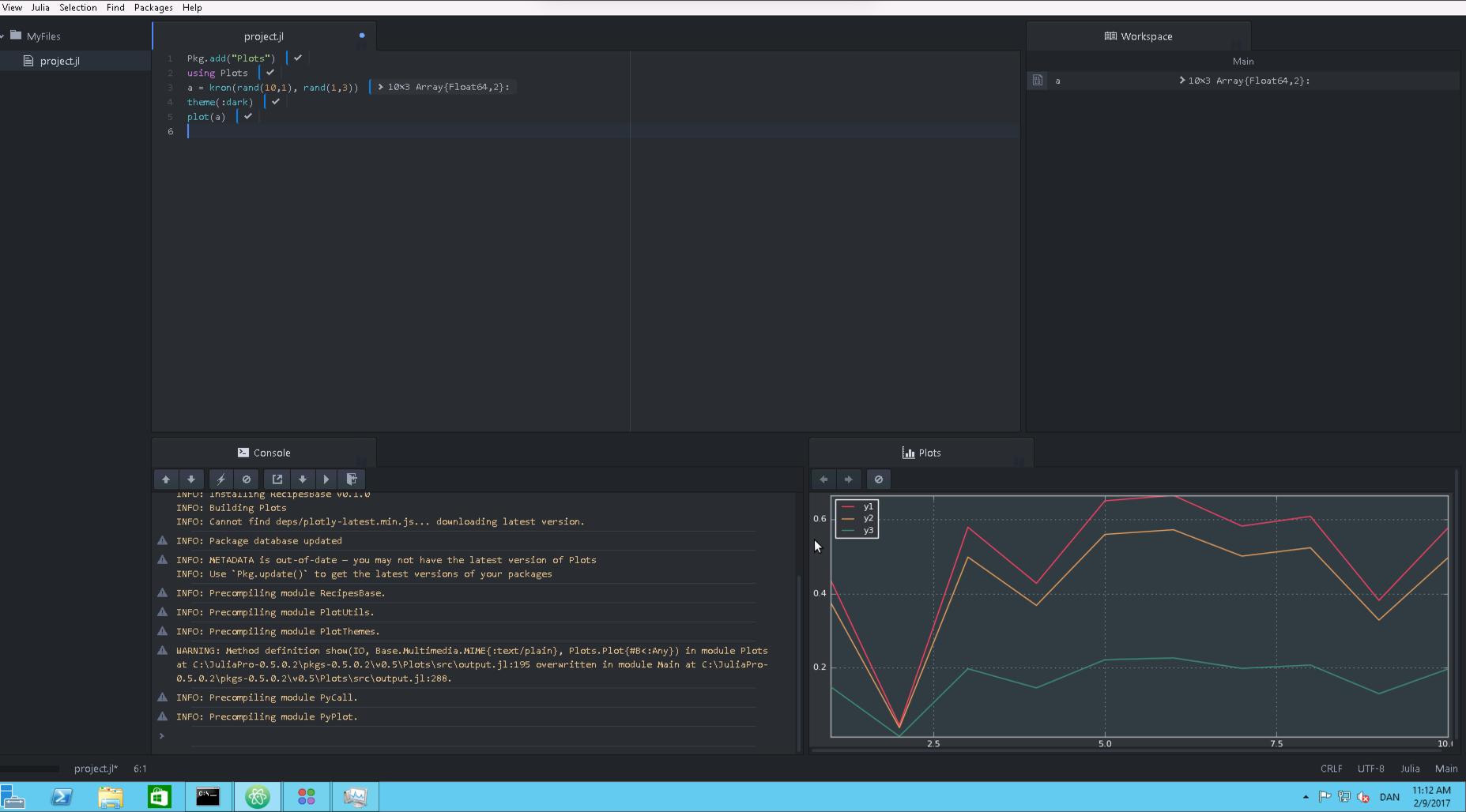
    Let’s try to open Juno, because… you’re worth it! (click to enlarge)

    I’m just adding  a package, loading it, creating some data, and plotting it (using a theme from PlotThemes.jl). Everything works fine, although I should note that Plots.jl took a while to load the first time around, as I’ve chosen the smallest VM available. Since we’re using JuliaPro, we could have been using Gadfly or PyPlot instead, and it would have been precompiled and ready to go.

    From here on, it’s up to you what to do. Analyse the stars, try out MXNet.jl, predict company defaults, or whatever you think is interesting.