Solving a simple discrete choice model using Gaussian quadrature

In the style of some of the earlier posts, I present a simple economic problem, that uses some sort of numerical method as part of the solution method. Of course, we use Julia to do so. However, this time we’re actually relying a bit on R, but don’t tell anyone.

Rust models

In the empirical discrete choice literature in economics, a relatively simple and popular framework is the one that matured in Rust (1987, 1988), and was later named Rust models in Aguirregabiria and Mira (2010). Basically, we consider an agent who has to choose a (in the infinite horizon) stationary policy (sequence of actions), to solve the following problem

\(\max_{a}E\left\{\sum_{t=0}^{T} \beta^t U(a_t, s_t)|s_0\right\}\)

where \(a=(a_0, a_1, \ldots, a_T)\), and \(s_t\) denotes the states. For simplicity, we consider binary decision problems such that \(a_t\in\{1,2\}\). Assume that there an additive shock, \(\varepsilon_t\), to utility such that

\(U(a_t,s_t)=U(a_t, x_t, \varepsilon_t) = u(a_t, x_t)+\varepsilon_t\)

where \(s_t=(x_t,\varepsilon_t)\) and \(x_t\) is usually called the observed states.

The additive and time separable nature of the problem allows us to consider a set of simpler problems instead. We reformulate the problem according to the principle of optimality, and write the problem in its dynamic programming formulation

\( V_t(x_t, \varepsilon_t) = max_{a_t}\left[u(a_t, x_t)+\epsilon_t + \beta E_{s_{t+1}|s_t}(V_{t+1}(x_{t+1}, \varepsilon_{t+1}))\right], \forall t\in\{0,1,\ldots,T\} \)

The object \(V_t\) is called the value function, as it summarizes the optimal value we can obtain. If we assume conditional independence between the observed states and the shocks along with the assumptions explained in the articles above, we can instead consider this simpler problem

\( W_t(x_t) = E_{\varepsilon_{t+1}|\varepsilon_t}\left\{max_{a_t}(u(a_t, x_t)+\varepsilon_t + \beta E_{x_{t+1}|x_t}((W_{t+1}(x_{t+1}))\right\}, \forall t\in\{0,1,\ldots,T\} \)

where \(W(x_t)\equiv E_{\varepsilon_{t+1}|\varepsilon}\left\{V_{t+1}(x_{t+1},\varepsilon_{t+1})\right\}\). This object is often called the ex-ante or integrated value function. Now, if we assume that the shocks are mean 0 extreme value type I, we get the following

\( W_t(x_t) = \log\left\{\sum_{a\in\mathcal{A}} \exp\left[u(a_t,x_t)+\beta E_{x_{t+1}|x_t}\left(W_{t+1}(x_{t+1})\right)\right]\right\}, \forall t\in\{0,1,\ldots,T\} \)

At this point we’re very close to something we can calculate. Either we just recursively apply the above to find the finite horizon solution, or if we’re in the infinite horizon case, then then we can come up with a guess for \(W\), and apply value function iterations (successive application of the right-hand side in the equation above), to find a solution. We just need to be able to handle the evaluation of the expected value inside the \(\exp\)‘s.

Solving for a continuous function

In the application below, we’re going to have a continuous state. Rust originally solved the problem of handling a continuous function on a computer by discretizing the continuous state in 90 or 175 bins, but we’re going to approach it a bit differently. We’re going to create a type that allows us to construct piecewise linear functions. This means that we’re going to have some nodes where we calculate the function value, and in between these, we simply use linear interpolation. Outside of the first and last nodes we simply set the value to the value at these nodes. We’re not going to extrapolate below, so this won’t be a problem.

Let us have a look at a type that can hold this information.

type PiecewiseLinear
    nodes
    values
    slopes
end

To construct an instance of this type from a set of nodes and a function, we’re going to use the following constructor

function PiecewiseLinear(nodes, f)
    slopes = Float64[]
    fn = f.(nodes)
    for i = 1:length(nodes)-1
        # node i and node i+1
        ni, nip1 = nodes[i], nodes[i+1]
        # f evaluated at the nodes
        fi, fip1 = fn[i], fn[i+1]
        # store slopes in each interval, so we don't have to recalculate them every time
        push!(slopes, (fip1-fi)/(nip1-ni))
    end
    # Construct the type
    PiecewiseLinear(nodes, fn, slopes)
end

Using an instance of \(PiecewiseLinear\) we can now evaluate the function at all input values between the first and last nodes. However, we’re going to have some fun with types in Julia. In Julia, we call a function using parentheses \(f(x)\), but we generally cannot call a type instance.

julia> pwl = PiecewiseLinear(1:10, sqrt)
PiecewiseLinear(1:10,[1.0,1.41421,1.73205,2.0,2.23607,2.44949,2.64575,2.82843,3.0,3.16228],[0.414214,0.317837,0.267949,0.236068,0.213422,0.196262,0.182676,0.171573,0.162278])
 
julia> pwl(3.5)
ERROR: MethodError: objects of type PiecewiseLinear are not callable

… but wouldn’t it be great if we could simply evaluate the interpolated function value at 3.5 that easily? We can, and it’s cool, fun, and extremely handy. The name of the concept is: call overloading. We simply need to define the behavior of “calling” (using parentheses with some input) an instance of a type.

function (p::PiecewiseLinear)(x)
    index_low = searchsortedlast(p.nodes, x)
    n = length(p.nodes)
    if 0 < index_low < n
        return p.values[index_low+1]+(x-p.nodes[index_low+1])*p.slopes[index_low]
    elseif index_low == n
        return p.values[end]
    elseif index_low == 0
        return p.values[1]
    end
end

Basically, we find out which interval we’re in, and then we interpolate appropriately in said interval. Let me say something upfront, or… almost upfront. This post is not about optimal performance. Julia is often sold as “the fast language”, but to me Julia is much more about productivity. Sure, it’s great to be able to optimize your code, but it’s also great to simply be able to do *what you want to do* – without too much hassle. Now, we can do what we couldn’t before.

julia> pwl(3.5)
1.8660254037844386

We can even plot it together with the actual sqrt function on the interval (2,4).

julia> using Plots
 
julia> plot(x->pwl(x), 2, 4, label="Piecewise Linear sqrt")
 
julia> plot!(sqrt, 2, 4, label="sqrt")
 
julia> savefig("sqrtfig")

and we get

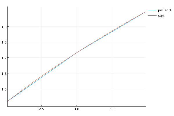
which seems to show a pretty good approximation to the square root function considering the very few nodes.

Numerical integrals using Gaussian quadrature

So we can now create continuous function approximations based on finite evaluation points (nodes). This is great, because this allow us to work with \(W\) in our code. The only remaining problem is: we need to evaluate the expected value of \(W\). This can be expressed as

\( E_x(f) = \int_a^b f(x)w(x)dx\)

where \(w(x)\) is going to be a probability density function and \(a\) and \(b\) can be finite or infinite and represent upper and lower bounds on the values the random variable (state) can take on. In the world of Gaussian quadrature, \(w\)‘s are called weight functions. Gaussian quadrature is basically a method for finding good evaluation points (nodes) and associated weights such that the following approximation is good

\(\int_a^b f(x)w(x)dx\approx \sum_{i=1}^N f(x_i)w_i\)

where \(N\) is the number of nodes. We’re not going to provide a long description of the methods involved, but we will note that the package DistQuads.jl allows us to easily obtain nodes and weights for a handful of useful distributions. To install this package write

Pkg.clone("https://github.com/pkofod/DistQuads.jl.git")

as it is not currently tagged in METADATA.jl. This is currently calling out to R’s statmod package. The syntax is quite simple. Define a distribution instance, create nodes and weights, and calculate the expected value of the function in three simple steps:

julia> using Distributions, DistQuads
 
julia> bd = Beta(1.5, 50.0)
Distributions.Beta{Float64}(α=1.5, β=50.0)
 
julia> dq = DistQuad(bd, N = 64)
DistQuads.DistQuad([0.000334965,0.00133945,0.00301221,0.0053512,0.00835354,0.0120155,0.0163327,0.0212996,0.0269103,0.03315780.738325,0.756581,0.774681,0.792633,0.810457,0.828194,0.845925,0.863807,0.882192,0.902105],[0.00484732,0.0184431,0.0381754,0.0603806,0.0811675,0.097227,0.106423,0.108048,0.102724,0.0920435  …  1.87035e-28,5.42631e-30,1.23487e-31,2.11992e-33,2.60541e-35,2.13019e-37,1.03855e-39,2.52575e-42,2.18831e-45,2.90458e-49],Distributions.Beta{Float64}(α=1.5, β=50.0))
 
julia> E(sqrt, dq)
0.15761865929803381

We can then try Monte Carlo integration with many nodes to see how close they are

julia> mean(sqrt.(rand(bd, 100000000)))
0.1576136243615477

and they appear to be in the same ballpark.

To replace, or not to replace

The model we’re considering here is a simple one. It’s a binary choice model very close to the model in Rust (1987). An agent is in charge of maintaining a bus fleet and has a binary choice each month then the buses come in for maintenance: replace the engine (effectively renewing the bus) or maintain it. Replacement costs a fixed price RC, and regular maintenance has a cost that is a linear function of the odometer reading since last replacement (or purchase if replacement has never occurred). We can use the expressions above to solve this model, but first we need to specify how the odometer reading changes from month to month conditional on the choices made. We assume that the odometer reading (mileage) changes according to the following

\(x_{t+1}=\tilde{a}x_{t}+(1-\tilde{a}x_t)\Delta x, \quad\text{where }\Delta x \sim Beta(1.4, 50.0)\)

where \(\tilde{a}=2-a\), and as we remember \(a\in\{1,2\}\). As we see, a replacement returns the state to 0 plus whatever mileage might accumulate that month, and regular maintenance means that the bus will end up with end of period mileage between \(x_{t+1}\) and 1. To give an idea about the state process, we see the pdf for the distribution of \(\Delta x\) below.

Solving the model

We are now ready to solve the model. Let us say that the planning horizon is 96 months and the monthly discount factor is 0.9. After the 96 months, the bus is scrapped at a value of 2 units of currency, such that

\(W_T(x)=2.0\)

and from here on, we use the recursion from above. First, set up the state space.

using Distributions, DistQuads, Plots
# State space
bd = Beta(1.5, 50.0)
dq = DistQuad(bd, N = 64)
 
Sˡ = 0
Sʰ = 1
 
n_nodes = 100 # arbitrary, but could be varied
nodes = linspace(Sˡ, Sʰ, n_nodes) # doesn't have to be uniformly distributed
 
RC = 11.5 # Replacement cost
c = 9.0 # parameter in linear maintenance cost c*x
β = 0.9 # discount factor

Then, define utility function and expectation operator

u1 = PiecewiseLinear(nodes, x->-c*x) # "continuous" cost of maintenance
u2 = PiecewiseLinear(nodes, x->-RC) # "continuous" cost of replacement (really just a number, but...)
 
# Expected value of f at x today given a where x′ is a possible state next period
Ex(f, x, a, dq) = E(x′->f((2-a)*x.+(Sʰ-(2-a)*x).*x′), dq)

Then, we simply

#### SOLVE
V = Array{PiecewiseLinear,1}(70)
V[70] = PiecewiseLinear(nodes, x->2)
for i = 69:-1:1
    EV1 = PiecewiseLinear(nodes, x->Ex(V[i+1], x, 1, dq))
    EV2 = PiecewiseLinear(nodes, x->Ex(V[i+1], x, 2, dq))
    V[i] = PiecewiseLinear(nodes, x->log(exp(u1(x)*EV1(x))+exp(u2(x)*EV2(x))))
end

To get our solution. We can then plot either integrated value functions or policies (choice probabilities). We calculate the policies using the following function

function CCP(x, i)
    EV1 = PiecewiseLinear(nodes, x->Ex(V[i], x, 1, dq))
    EV2 = PiecewiseLinear(nodes, x->Ex(V[i], x, 2, dq))
    1/(1+exp(u2(x)*EV2(x)-u1(x)*EV1(x)))
end


We see that there are not 69/70 distinct curves in the plots. This is because we eventually approach the “infinite horizon”/stationary policy and solution.

Simulation

Given the CCPs from above, it is very straight forward to simulate an agent say from period 1 to period 69.

#### SIMULATE
x0 = 0.0
x = [x0]
a0 = 0
a = [a0]
T = 69
for i = 2:T
   _a = rand()<CCP(x[end], i) ? 1 : 2
   push!(a, _a)
   push!(x, (2-_a)*x[end]+(Sʰ-(2-_a)*x[end])*rand(bd))
end
plot(1:T, x, label="mileage")
Is = []
for i in eachindex(a)
    if a[i] == 2
        push!(Is, i)
    end
end
vline!(Is, label="replacement")


Conclusion
This blog post had a look at simple quadrature, creating custom types with call overloading in Julia, and how this can be used to a solve a very simple discrete choice model in Julia. Interesting extensions are of course to allow for more states, more choices, other shock distributions than extreme value type I and so on. Let me know if you try to extend the model in any of those directions, and I would love to have a look!

References

  • Aguirregabiria, Victor, and Pedro Mira. “Dynamic discrete choice structural models: A survey.” Journal of Econometrics 156.1 (2010): 38-67.
  • Rust, John. “Optimal replacement of GMC bus engines: An empirical model of Harold Zurcher.” Econometrica: Journal of the Econometric Society (1987): 999-1033.
  • John, Rust. “Maximum likelihood estimation of discrete control processes.” SIAM Journal on Control and Optimization 26.5 (1988): 1006-1024.
  • DynProg Class – Week 2

    This post, and other posts with similar tags and headers, are mainly directed at the students who are following the Dynamic Programming course at Dept. of Economics, University of Copenhagen in the Spring 2017. The course is taught using Matlab, but I will provide a few pointers as to how you can use Julia to solve the same problems. So if you are an outsider reading this I welcome you, but you won’t find all the explanations and theory here. If you want that, you’ll have to come visit us at UCPH and enroll in the class!

    This week we continue with a continuous choice model. This means we have to use interpolation and numerical optimization.

    A (slightly less) simple model

    Consider a simple continuous choice consumption-savings model:

    \(V_t(M_t) = \max_{C_t}\sqrt{C_t}+\mathbb{E}[V_{t+1}(M_{t+1})|C_t, M_t]\)
    subject to
    \(M_{t+1} = M_t – C_t+R_t\\
    C_t\leq M_t\\
    C_t\in\mathbb{R}_+\)

    where \(R_t\) is 1 with probability \(\pi\) and 0 with probability \(1-\pi\), \(\beta=0.9\), and \(\bar{M}=5\)

    Last week the maximization step was merely comparing values associated with the different discrete choices. This time we have to do continuous optimization in each time period. Since the problem is now continuous, we cannot solve for all \(M_t\). Instead, we need to solve for \(V_t\) at specific values of \(M_t\), and interpolate in between. Another difference to last time is the fact that the transitions are stochastic, so we need to form (very simple) expectations as part of the Bellman equation evaluations.

    Interpolation

    It is of course always possible to make your own simple interpolation scheme, but we will use the functionality provided by the Interpolations.jl package. To perform interpolation, we need a grid to be used for interpolation \(\bar{x}\), and calculate the associated function values.

    f(x) = (x-3)^2
    x̄ = linspace(1,5,5)
    fx̄ = f.()

    Like last time, we remember that the dot after the function name and before the parentheses represent a “vectorized” call, or a broadcast – that is we call f on each element of the input. We now use the Interpolations.jl package to create an interpolant \(\hat{f}\).

    using Interpolations
    f̂ = interpolate((collect(),), fx̄, Gridded(Linear()))

    We can now index into \(\hat{f}\) as if it was an array

    [-3] #returns 16.0

    We can also plot it

    using Plots
    plot()

    which will output

    Solving the model

    Like last time, we prepare some functions, variables, and empty containers (Arrays)

    # Model again
    u(c) = sqrt(c)
    T = 10; β = 0.9
    π = 0.5 ;M₁ = 5
    # Number of interpolation nodes
    Nᵐ = 50 # number of grid points in M grid
    Nᶜ  = 50 # number of grid points in C grid
     
    M = Array{Vector{Float64}}(T)
    V = Array{Any}(T)
    C = Array{Any}(T)

    The V and C arrays are allocated using the type “Any”. We will later look at how this can hurt performance, but for now we will simply do the convenient thing. Then we solve the last period

    M[T] = linspace(0,M₁+T,Nᵐ)
    C[T] = M[T]
    V[T] = interpolate((M[T],), u.(C[T]), Gridded(Linear()))

    This new thing here is that we are not just saving V[T] as an Array. The last element is the interpolant, such that we can simply index into V[T] as if we had the exact solution at all values of M (although we have to remember that it is an approximation). For all periods prior to T, we have to find the maximum as in the Bellman equation from above. To solve this reduced “two-period” problem (sum of utility today and discounted value tomorrow), we need to form expectations over the two possible state transitions given an M and a C today, and then we need to find the value of C that maximizes current value. We define the following function to handle this

    # Create function that returns the value given a choice, state, and period
    v(c, m, t, V) = u(c)*(π*V[t+1][m-c+1]+(1)*V[t+1][m-c])

    Notice how convenient it is to simply index into V[t] using the values we want to evaluate tomorrow’s value function at. We perform the maximization using grid search on a predefined grid from 0 to the particular M we’re solving form. If we abstract away from the interpolation step, this is exactly what we did last time.

    for t = T-1:-1:1
        M[t] = linspace(0,M₁+t,Nᵐ)
        C[t] = zeros(M[t])
        Vt = fill(-Inf, length(M[t]))
        for (iₘ, m) = enumerate(M[t])
            for c in linspace(0, m, Nᶜ)
                _v = v(c, m, t, V)
                if _v >= Vt[iₘ]
                    Vt[iₘ] = _v
                    C[t][iₘ] = c
                end
            end
        end
        V[t] = interpolate((M[t],), Vt, Gridded(Linear()))
    end

    Then we can plot the value functions to verify that they look sensible

    Nicely increasing in time and in M.

    Using Optim.jl for optimization

    The last loop could just as well have been done using a proper optimization routine. This will in general be much more robust, as we don’t confine ourselves to a certain amount of C-values. We use the one of the procedures in Optim.jl. In Optim.jl, constrained, univariate optimization is available as either Brent’s method or Golden section search. We will use Brent’s method. This is the standard method, so an optimization call simply has the following syntax

    using Optim
    f(x) = x^2
    optimize(f, -1.0, 2.0)

    Unsurprisingly, this will return the global minimizer 0.0. However, if we constrain ourselves to a strictly positive interval

    optimize(f, 1.0, 2.0)

    we get a minimizer of 1.0. This is not the unconstrained minimizer of the square function, but it is minimizer given the constraints. Then, it should be straight forward to see how the grid search loop can be converted to a loop using optimization instead.

    for t = T-1:-1:1
        update_M!(M, M₁, t, Nᵐ)
        C[t] = zeros(M[t])
        Vt = fill(-Inf, length(M[t]))
        for (iₘ, m) = enumerate(M[t])
            if m == 0.0
                C[t][iₘ] = m
                Vt[iₘ] = v(m, m, t, V)
            else
                res = optimize(c->-v(c, m, t, V), 0.0, m)
                Vt[iₘ] = -Optim.minimum(res)
                C[t][iₘ] = Optim.minimizer(res)
            end
        end
        V[t] = interpolate((M[t],), Vt, Gridded(Linear()))
    end

    If our agent has no resources at the beginning of the period, the choice set has only one element, so we skip the optimization step. We also have to negate the minimum to get the maximum we’re looking for. The main advantage of using a proper optimization routine is that we’re not restricting C to be in any predefined grid. This increases precision. If we look at the number of calls to “v” (using Optim.f_calls(res)), we see that it generally takes around 10-30 v calls. With only 10-30 grid points from 0 up to M, we would generally get an approximate solution of much worse quality.

    Julia bits and pieces

    This time we used a few different package from the Julia ecosystem: Plots.jl, Interpolations.jl, and Optim.jl. These are based on my personal choices (full disclosure: I’ve contributed to the first and the last), but there are lots of packages to explore. Visit the JuliaLang discourse forum or gitter channel to discuss Julia and the various packages with other users.

    DynProg Class – Week 1

    This post, and other posts with similar tags and headers, are mainly directed at the students who are following the Dynamic Programming course at Dept. of Economics, University of Copenhagen in the Spring 2017. The course is taught using Matlab, but I will provide a few pointers as to how you can use Julia to solve the same problems. So if you are an outsider reading this I welcome you, but you won’t find all the explanations and theory here. Then you’ll have to come visit us at UCPH and enroll in the class!

    We start out with very simple examples and Julia code, and gradually ramp up the difficulty level.

    Simple model

    Consider the simplest consumption-savings model:

    \(V^*(M) = \max_{C_1,C_2,\ldots,C_T}\beta^0\sqrt{C_1},\beta^1\sqrt{C2},\ldots,\beta^T\sqrt{C_T}\)

    subject to
    $$\bar{M} = C_1+C_2+\ldots+C_T\equiv m_1$$
    $$m_{t+1} = m_t – C_t$$
    $$C_t\in\mathbb{N}$$
    $$\beta=0.9,\quad\bar{M}=5$$

    Let us try to solve such models.

    1) Brute force

    This is not a very clever way, but let us start somewhere. We don’t have a better method – yet! Set T=2. Note, there is only one free choice to vary. Given some consumption in period t, the other is given due to the “No cake left” boundary condition.

        # Primitives
        β = 0.90
        α = 0.5
        u(x, α) = x^α
        ## State
        M̄ = 5.0
        Cᵒᵖᵗ = u(0.0, α) + β*u(M̄, α)
        Vᵒᵖᵗ = -Inf
        for C1 in 1.0:1.0:M̄
            V = u(C1, α) + β*u(M̄-C1, α)
            if Vᵒᵖᵗ &lt;= V
                Vᵒᵖᵗ = V
                Cᵒᵖᵗ = C1
            end
        end
        println("Results")
        println("* optimimum: ", Vᵒᵖᵗ)
        println("* optimizer: ", Cᵒᵖᵗ)

    This tells us that our agent should consume three units in the first period and two in the last period.

    2) Vary β and M

    Check that different M’s and β’s give sensible predictions.

    We don’t want to rerun that code manually each time – we’re going to need something smarter. Let’s wrap it in a function. In Julia, a typical function (method) definition looks something like the following.

    function brute_force(M̄, α, β)
        Vᵒᵖᵗ = u(0.0, α) + β*u(M̄, α)
        Cᵒᵖᵗ = 0 
     
        for C1 in 1.0:1.0:M̄
            V = u(C1, α) + β*u(M̄-C1, α)
            if Vᵒᵖᵗ <= V
                Vᵒᵖᵗ = V
                Cᵒᵖᵗ = C1
            end
        end
        Vᵒᵖᵗ, Cᵒᵖᵗ
    end

    Notice that whatever is on the last line will be returned. For example, you can verify that it returns the same thing as the loop above, or check what happens if β is 0:

    brute_force(M̄, α, 0.0)

    The output tells us that the agent should consume everything in the first period. This is consistent with the intuition that the agent doesn’t care about the future at all. What if we have no units at the first period?

    brute_force(0, α, β)

    We see that the agent should consume nothing. This might seem like a stupid thing to test for, but it is always important to sanity check your code. If it can’t predict things that are obvious, it will probably also give wrong answers to more complex cases. It can be hard to come up with such cases, but the last two examples will always hold. Full discounting -> full consumption today. No ressources -> no consumption today (unless you can borrow).

    3) Solve a model using backwards induction

    It requires little convincing to realize, that it is wasteful to check all possible combinations – especially when the number of periods increases. Instead, we use the principle of optimality to solve the problem using dynamic programming. To solve the model using dynamic programming, we need to create a few variables to hold the value and policy functions. These will hold the solutions from each (t,m) subproblem. We start with T=3

    T = 3
    M = 0.0:M̄
    Vᵒᵖᵗ = [zeros(M) for t = 1:T]
    Cᵒᵖᵗ = [zeros(M) for t = 1:T]

    We’ve used vectors of vectors here, but could just as well have created a $5\times 3$ matrix in this case. However, in a more general class of models, the number of states might vary over time, and there a vector of vector becomes convenient. With these variables in place, we can solve the last period by realizing that given some resource level in period T, we need to consume everything in order fulfill the constraints of the problem (no cake left on the table!).

    Vᵒᵖᵗ[end] = sqrt.(M)
    Cᵒᵖᵗ[end] = M

    Notice the dot after sqrt. This is Julia syntax for “broadcast the square root function over M”. Then, we solve for the period t=T-1, then t=T-2, and then we’re done. We implement a straight forward loop over all possible m’s and feasible consumption given these m’s, by using the fact that the feasible values for consumption make up the set
    $$\{0,1,2,…,m_t\}$$.

    for t = T-1:-1:1
        for imₜ = 1:length(M)
            Vᵒᵖᵗ[t][imₜ] = -Inf # some value lower than sqrt(0)
            for (icₜ,cₜ) = enumerate(0:M[imₜ])
                v = u(cₜ, α) + β*Vᵒᵖᵗ[t+1][1+imₜ-icₜ]
                if v > Vᵒᵖᵗ[t][imₜ]
                    Vᵒᵖᵗ[t][imₜ] = v
                    Cᵒᵖᵗ[t][imₜ] = cₜ
                end
            end
        end
    end
    println("Results")
    println("* optimimum: ", Vᵒᵖᵗ)
    println("* optimizer: ", Cᵒᵖᵗ)

    Again, you should try to see if some of all this shouldn’t really be separate functions.

    Julia bits and pieces

    To close off this post, let me just briefly touch upon some of the things we used above, that might be different from Matlab. To allocate an empty array, write

    V = Vector(10)

    or a vector with some specific element value (here, a Float64 NaN)

    W = fill(NaN, 10)

    Indexing into arrays is done with square brackets. For example, let’s assign the first element of W to a variable WW

    WW = W[1]

    And the same goes for setting the value at some index

    W[1] = 0.4;
    W

    Functions are define using either short or long form

    function f(x,y)
        x+y+rand() # returns the sum of the two inputs and a random number
    end
    g(x,y) = x+y+rand()

    and comments are inserted using # or the #= =# blocks

    # This is a comment
     
    #= This
    is
    a
    comment
    =#

    For-loops are written as

    for a = some_iterator
        # do something
    end

    or to get both the value and a counter use enumerate

    for (i, a) = enumerate(some_iterator)
        # do stuff with a and index something with i
    end

    Code that should be run conditional on some statement being true is written as

    if condition
        # do something if condition is satisfied
    end

    and that’s all for now, folks!